Capacitively Coupled Charge Qubits: Difference between revisions
| (15 intermediate revisions by the same user not shown) | |||
| Line 1: | Line 1: | ||
This project started in the Fall of 2014, focusing on the operation of two or more charge qubits which are capacitively coupled. |
This project started in the Fall of 2014, focusing on the operation of two or more charge qubits which are capacitively coupled. Current PDF Summary can be found [[File:Capacitively Coupled Qubits.pdf]] |
||
==General Formulation== |
==General Formulation== |
||
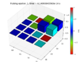
[[Image:Detuning graph.png|thumb|Energy levels of the 2 qubit system as a function of both detunings.|300px]] |
[[Image:Detuning graph.png|thumb|Energy levels of the 2 qubit system as a function of both detunings.|300px]] |
||
| Line 40: | Line 40: | ||
<math> |
<math> |
||
\lambda_1 = -\sqrt{\Delta_1^2+\Delta_2^2+\frac{\epsilon_1^2}{4}+g^2+\sqrt{4\Delta_1^2\Delta_2^2+\epsilon_1^2(\Delta_2+g^2)}} |
\lambda_1 = -\sqrt{\Delta_1^2+\Delta_2^2+\frac{\epsilon_1^2}{4}+g^2+\sqrt{4\Delta_1^2\Delta_2^2+\epsilon_1^2(\Delta_2^2+g^2)}} |
||
</math> |
</math> |
||
<math> |
<math> |
||
\lambda_2 = -\sqrt{\Delta_1^2+\Delta_2^2+\frac{\epsilon_1^2}{4}+g^2-\sqrt{4\Delta_1^2\Delta_2^2+\epsilon_1^2(\Delta_2+g^2)}} |
\lambda_2 = -\sqrt{\Delta_1^2+\Delta_2^2+\frac{\epsilon_1^2}{4}+g^2-\sqrt{4\Delta_1^2\Delta_2^2+\epsilon_1^2(\Delta_2^2+g^2)}} |
||
</math> |
</math> |
||
<math> |
<math> |
||
\lambda_3 = \sqrt{\Delta_1^2+\Delta_2^2+\frac{\epsilon_1^2}{4}+g^2-\sqrt{4\Delta_1^2\Delta_2^2+\epsilon_1^2(\Delta_2+g^2)}} |
\lambda_3 = \sqrt{\Delta_1^2+\Delta_2^2+\frac{\epsilon_1^2}{4}+g^2-\sqrt{4\Delta_1^2\Delta_2^2+\epsilon_1^2(\Delta_2^2+g^2)}} |
||
</math> |
</math> |
||
<math> |
<math> |
||
\lambda_4 = \sqrt{\Delta_1^2+\Delta_2^2+\frac{\epsilon_1^2}{4}+g^2+\sqrt{4\Delta_1^2\Delta_2^2+\epsilon_1^2(\Delta_2+g^2)}} |
\lambda_4 = \sqrt{\Delta_1^2+\Delta_2^2+\frac{\epsilon_1^2}{4}+g^2+\sqrt{4\Delta_1^2\Delta_2^2+\epsilon_1^2(\Delta_2^2+g^2)}} |
||
</math> |
</math> |
||
which to second order in <math>\epsilon_1</math> are: |
which to second order in <math>\epsilon_1</math> are: |
||
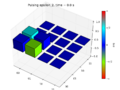
[[Image:Second order.png|thumb|Energy gap between 01 and 10 states as a function of both detunings. Here, <math>\Delta_1 = 2</math>,<math>\Delta_2 = 1</math>, and <math>g = 1</math>, so the gap is invariant to second-order fluctuations in <math>\epsilon_1</math>.|300px]] |
|||
<math> |
<math> |
||
| Line 62: | Line 64: | ||
<math> |
<math> |
||
\lambda_2 \approx \lambda_2^0 + \frac{\Delta_2(\Delta_1 |
\lambda_2 \approx \lambda_2^0 + \frac{\Delta_2(\Delta_1-\Delta_2)-g^2}{8\Delta_1\Delta_2\lambda_2^0}\epsilon_1^2 |
||
</math> |
</math> |
||
<math> |
<math> |
||
\lambda_3 \approx \lambda_3^0 + \frac{\Delta_2(\Delta_1 |
\lambda_3 \approx \lambda_3^0 + \frac{\Delta_2(\Delta_1-\Delta_2)-g^2}{8\Delta_1\Delta_2\lambda_3^0}\epsilon_1^2 |
||
</math> |
</math> |
||
| Line 76: | Line 78: | ||
<math> |
<math> |
||
g^2 = \Delta_2(\Delta_1 |
g^2 = \Delta_2(\Delta_1-\Delta_2) |
||
</math> |
</math> |
||
Unfortunately, none of the other transitions can be made to be invariant to second order fluctuations in <math>\epsilon_1</math>. Also, If we wish to make this transition invariant to all second order detuning fluctuations, we must set <math>\Delta_1 = \Delta_2</math>, making <math>g = 0</math>. |
|||
<math> |
|||
g^2 = \frac{1}{2\Delta_2}(\Delta_1+\Delta_2)\sqrt{(\Delta_1+\Delta_2)(\Delta_1^3-\Delta_1^2\Delta_2+3\Delta_1\Delta_2^2+\Delta_2^3)}-\Delta_1^3-\Delta_1^2\Delta_2-\Delta_1\Delta_2^2-\Delta_2^3 |
|||
</math> |
|||
===Tunnel Coupling and Capacitive Coupling Noise=== |
===Tunnel Coupling and Capacitive Coupling Noise=== |
||
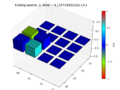
[[Image:equal_deltas.png|thumb|Energy gap between 01 and 10 states as a function of both detunings. Here, <math>\Delta_1= \Delta_2 = 1</math>. Although the second order effects of the detunings are non-zero, they are relatively small.|300px]] |
|||
Assuming that we sit at the sweet spot <math>\epsilon_1 = \epsilon_2 = 0</math>, the energies are relatively simple, so we can easily see the effect of noise on the other parameters. |
Assuming that we sit at the sweet spot <math>\epsilon_1 = \epsilon_2 = 0</math>, the energies are relatively simple, so we can easily see the effect of noise on the other parameters. |
||
| Line 103: | Line 102: | ||
|} |
|} |
||
Note that if we want any of the transitions to be invariant to first-order fluctuations in tunnel coupling, we would need to set <math>\Delta_1 |
Note that if we want any of the transitions to be invariant to first-order fluctuations in tunnel coupling, we would need to set either <math>\Delta_1</math> or <math>\Delta_2</math> to zero or set <math>\Delta_1 = \Delta_2</math>. The first change would make the energy levels degenerate, which must be avoided. If we set the tunnel couplings to be equal, it would be impossible to make any of the transitions invariant to second order effects in the detuning. |
||
There is nothing we can do short of making the energy levels degenerate to make the transitions invariant with respect to first-order fluctuations in capacitive coupling. We could, however, make the coupling itself as stable as possible through manipulating the geometry of the system. |
|||
==Rotations== |
==Rotations== |
||
'''SECTION IN PROGRESS''' |
|||
===Shifting to the Rotating Frame=== |
|||
After bringing the system adiabatically to the sweet spot <math>\epsilon_1=\epsilon_2=0</math>, we can apply an AC pulse to some of our parameters to induce a rotation within the system. |
After bringing the system adiabatically to the sweet spot <math>\epsilon_1=\epsilon_2=0</math>, we can apply an AC pulse to some of our parameters to induce a rotation within the system. |
||
| Line 124: | Line 122: | ||
0 & 0 & 0 & -B |
0 & 0 & 0 & -B |
||
\end{matrix}\right)\cos{(\omega_{AC}t)}</math> || <math>\frac{1}{2}\left( \begin{matrix} |
\end{matrix}\right)\cos{(\omega_{AC}t)}</math> || <math>\frac{1}{2}\left( \begin{matrix} |
||
0 & A_1 & A_2 & 0 \\ |
0 & A_1\times\text{Sign}(\Delta_1-\Delta_2) & -A_2 & 0 \\ |
||
A_1\times\text{Sign}(\Delta_1-\Delta_2) & 0 & 0 & -A_2\times\text{Sign}(\Delta_1-\Delta_2) \\ |
|||
A_1 & 0 & 0 & A_3 \\ |
|||
A_2 & 0 & 0 & |
-A_2 & 0 & 0 & -A_1 \\ |
||
0 & -A_2\times\text{Sign}(\Delta_1-\Delta_2) & -A_1 & 0 |
|||
0 & A_3 & A_4 & 0 |
|||
\end{matrix}\right)\cos{(\omega_{AC}t)}</math> |
\end{matrix}\right)\cos{(\omega_{AC}t)}</math> |
||
|- |
|- |
||
| Line 136: | Line 134: | ||
0 & 0 & 0 & -B |
0 & 0 & 0 & -B |
||
\end{matrix}\right)\cos{(\omega_{AC}t)}</math> || <math>\frac{1}{2}\left( \begin{matrix} |
\end{matrix}\right)\cos{(\omega_{AC}t)}</math> || <math>\frac{1}{2}\left( \begin{matrix} |
||
0 & |
0 & -C_1\times\text{Sign}(\Delta_1-\Delta_2) & -C_2 & 0 \\ |
||
-C_1\times\text{Sign}(\Delta_1-\Delta_2) & 0 & 0 & C_2\times\text{Sign}(\Delta_1-\Delta_2) \\ |
|||
0 & 0 & 0 &B \\ |
|||
-C_2 & 0 & 0 & -C_1 \\ |
|||
0 & |
0 & C_2\times\text{Sign}(\Delta_1-\Delta_2) & -C_1 & 0 |
||
\end{matrix}\right)\cos{(\omega_{AC}t)}</math> |
\end{matrix}\right)\cos{(\omega_{AC}t)}</math> |
||
|- |
|- |
||
| Line 149: | Line 147: | ||
\end{matrix}\right)\cos{(\omega_{AC}t)}</math> || <math>\frac{1}{2}\left( \begin{matrix} |
\end{matrix}\right)\cos{(\omega_{AC}t)}</math> || <math>\frac{1}{2}\left( \begin{matrix} |
||
-B\frac{\Delta_1+\Delta_2}{\lambda_1} & 0 & 0 & -B\frac{g}{\lambda_1} \\ |
-B\frac{\Delta_1+\Delta_2}{\lambda_1} & 0 & 0 & -B\frac{g}{\lambda_1} \\ |
||
0 & -B\frac{\Delta_1-\Delta_2}{\lambda_2} & -B\frac{g}{\lambda_2} & 0 \\ |
0 & -B\frac{\Delta_1-\Delta_2}{\lambda_2} & -B\frac{g}{\lambda_2}\times\text{Sign}(\Delta_1-\Delta_2) & 0 \\ |
||
0& -B\frac{g}{\lambda_2} & B\frac{\Delta_1-\Delta_2}{\lambda_2} & 0\\ |
0& -B\frac{g}{\lambda_2}\times\text{Sign}(\Delta_1-\Delta_2) & B\frac{\Delta_1-\Delta_2}{\lambda_2} & 0\\ |
||
-B\frac{g}{\lambda_1}& 0 & 0 &B\frac{\Delta_1+\Delta_2}{\lambda_1} |
-B\frac{g}{\lambda_1}& 0 & 0 &B\frac{\Delta_1+\Delta_2}{\lambda_1} |
||
\end{matrix}\right)\cos{(\omega_{AC}t)}</math> |
\end{matrix}\right)\cos{(\omega_{AC}t)}</math> |
||
| Line 160: | Line 158: | ||
0 & 0 & B & 0 |
0 & 0 & B & 0 |
||
\end{matrix}\right)\cos{(\omega_{AC}t)}</math> || <math>\frac{1}{2}\left( \begin{matrix} |
\end{matrix}\right)\cos{(\omega_{AC}t)}</math> || <math>\frac{1}{2}\left( \begin{matrix} |
||
-B\frac{\Delta_1+\Delta_2}{\lambda_1} & 0 & 0 & -B\frac{g}{\lambda_1} \\ |
|||
0 & 0 & B & 0 \\ |
|||
0 & B\frac{\Delta_1-\Delta_2}{\lambda_2} & B\frac{g}{\lambda_2}\times\text{Sign}(\Delta_1-\Delta_2) & 0 \\ |
|||
0 & 0 & 0 &B \\ |
|||
0 & B\frac{g}{\lambda_2}\times\text{Sign}(\Delta_1-\Delta_2) & -B\frac{\Delta_1-\Delta_2}{\lambda_2} & 0 \\ |
|||
B & 0 & 0 & 0 \\ |
|||
-B\frac{g}{\lambda_1}& 0 & 0 &B\frac{\Delta_1+\Delta_2}{\lambda_1} |
|||
0 & B & 0 & 0 |
|||
\end{matrix}\right)\cos{(\omega_{AC}t)}</math> |
\end{matrix}\right)\cos{(\omega_{AC}t)}</math> |
||
|} |
|} |
||
where <math>\lambda_1 = \sqrt{(\Delta_1+\Delta_2)^2+g^2}</math>, <math>\lambda_2 = \sqrt{(\Delta_1-\Delta_2)^2+g^2}</math>, and <math>A_1</math>, <math>A_2</math>, <math>C_1</math>, and <math>C_2</math> are all complicated functions of the parameters which are discussed below. |
|||
Based off of the rotation matrices in the energy basis, it's clear that the situation in which <math>\Delta_1>\Delta_2</math> fundamentally differs from the case in which <math>\Delta_1<\Delta_2</math>. Moreover, it can be seen that the case in which <math>\Delta_1=\Delta_2</math> yields diverging results (as some of the matrix elements feature a step function at this point). So in practice, it would be good to avoid this point. Writing the rotations explicitly for the two regimes: |
|||
{| border="1" cellpadding="2" |
|||
!width="50"|AC Pulse |
|||
!width="225"|Energy Basis (<math>\Delta_1>\Delta_2</math>) |
|||
!width="225"|Energy Basis (<math>\Delta_1<\Delta_2</math>) |
|||
|- |
|||
|<math>\epsilon_1</math> || <math>\frac{1}{2}\left( \begin{matrix} |
|||
0 & A_1 & -A_2 & 0 \\ |
|||
A_1 & 0 & 0 & -A_2 \\ |
|||
-A_2 & 0 & 0 & -A_1 \\ |
|||
0 & -A_2 & -A_1 & 0 |
|||
\end{matrix}\right)\cos{(\omega_{AC}t)}</math> || <math>\frac{1}{2}\left( \begin{matrix} |
|||
0 & -A_1 & -A_2 & 0 \\ |
|||
-A_1 & 0 & 0 & A_2 \\ |
|||
-A_2 & 0 & 0 & -A_1 \\ |
|||
0 & A_2 & -A_1 & 0 |
|||
\end{matrix}\right)\cos{(\omega_{AC}t)}</math> |
|||
|- |
|||
|<math>\epsilon_2</math> || <math>\frac{1}{2}\left( \begin{matrix} |
|||
0 & -C_1 & -C_2 & 0 \\ |
|||
-C_1 & 0 & 0 & C_2 \\ |
|||
-C_2 & 0 & 0 & -C_1 \\ |
|||
0 & C_2 & -C_1 & 0 |
|||
\end{matrix}\right)\cos{(\omega_{AC}t)}</math> || <math>\frac{1}{2}\left( \begin{matrix} |
|||
0 & C_1 & -C_2 & 0 \\ |
|||
C_1 & 0 & 0 & -C_2 \\ |
|||
-C_2 & 0 & 0 & -C_1 \\ |
|||
0 & -C_2 & -C_1 & 0 |
|||
\end{matrix}\right)\cos{(\omega_{AC}t)}</math> |
|||
|- |
|||
|<math>\Delta_1</math> || <math>\frac{1}{2}\left( \begin{matrix} |
|||
-B\frac{\Delta_1+\Delta_2}{\lambda_1} & 0 & 0 & -B\frac{g}{\lambda_1} \\ |
|||
0 & -B\frac{\Delta_1-\Delta_2}{\lambda_2} & -B\frac{g}{\lambda_2} & 0 \\ |
|||
0& -B\frac{g}{\lambda_2} & B\frac{\Delta_1-\Delta_2}{\lambda_2} & 0\\ |
|||
-B\frac{g}{\lambda_1}& 0 & 0 &B\frac{\Delta_1+\Delta_2}{\lambda_1} |
|||
\end{matrix}\right)\cos{(\omega_{AC}t)}</math> || <math>\frac{1}{2}\left( \begin{matrix} |
|||
-B\frac{\Delta_1+\Delta_2}{\lambda_1} & 0 & 0 & -B\frac{g}{\lambda_1} \\ |
|||
0 & -B\frac{\Delta_1-\Delta_2}{\lambda_2} & B\frac{g}{\lambda_2} & 0 \\ |
|||
0& B\frac{g}{\lambda_2} & B\frac{\Delta_1-\Delta_2}{\lambda_2} & 0\\ |
|||
-B\frac{g}{\lambda_1}& 0 & 0 &B\frac{\Delta_1+\Delta_2}{\lambda_1} |
|||
\end{matrix}\right)\cos{(\omega_{AC}t)}</math> |
|||
|- |
|||
|<math>\Delta_2</math> || <math>\frac{1}{2}\left( \begin{matrix} |
|||
-B\frac{\Delta_1+\Delta_2}{\lambda_1} & 0 & 0 & -B\frac{g}{\lambda_1} \\ |
|||
0 & B\frac{\Delta_1-\Delta_2}{\lambda_2} & B\frac{g}{\lambda_2} & 0 \\ |
|||
0 & B\frac{g}{\lambda_2} & -B\frac{\Delta_1-\Delta_2}{\lambda_2} & 0 \\ |
|||
-B\frac{g}{\lambda_1}& 0 & 0 &B\frac{\Delta_1+\Delta_2}{\lambda_1} |
|||
\end{matrix}\right)\cos{(\omega_{AC}t)}</math> || <math>\frac{1}{2}\left( \begin{matrix} |
|||
-B\frac{\Delta_1+\Delta_2}{\lambda_1} & 0 & 0 & -B\frac{g}{\lambda_1} \\ |
|||
0 & B\frac{\Delta_1-\Delta_2}{\lambda_2} & -B\frac{g}{\lambda_2} & 0 \\ |
|||
0 & -B\frac{g}{\lambda_2} & -B\frac{\Delta_1-\Delta_2}{\lambda_2} & 0 \\ |
|||
-B\frac{g}{\lambda_1}& 0 & 0 &B\frac{\Delta_1+\Delta_2}{\lambda_1} |
|||
\end{matrix}\right)\cos{(\omega_{AC}t)}</math> |
|||
|} |
|||
We can further analyze these matrices by considering the effective rotations in the rotating frame for different applied frequencies, using the rotating wave approximation: |
|||
{| border="1" cellpadding="2" |
|||
! colspan="2" width="100"|AC Pulse |
|||
!width="225"|Rotating Frame (<math>\Delta_1>\Delta_2</math>) |
|||
!width="225"|Rotating Frame (<math>\Delta_1<\Delta_2</math>) |
|||
|- |
|||
|rowspan="2"|<math>\epsilon_1</math> || <math>\omega_{AC} = (\lambda_1-\lambda_2)/\hbar</math> || <math>\frac{1}{4}\left( \begin{matrix} |
|||
0 & A_1 & 0 & 0 \\ |
|||
A_1 & 0 & 0 & 0 \\ |
|||
0 & 0 & 0 & -A_1 \\ |
|||
0 & 0 & -A_1 & 0 |
|||
\end{matrix}\right)</math> || <math>\frac{1}{4}\left( \begin{matrix} |
|||
0 & -A_1 & 0 & 0 \\ |
|||
-A_1 & 0 & 0 & 0 \\ |
|||
0 & 0 & 0 & -A_1 \\ |
|||
0 & 0 & -A_1 & 0 |
|||
\end{matrix}\right)</math> |
|||
|- |
|||
|<math>\omega_{AC} = (\lambda_1+\lambda_2)/\hbar</math> || <math>\frac{1}{4}\left( \begin{matrix} |
|||
0 & 0 & -A_2 & 0 \\ |
|||
0 & 0 & 0 & -A_2 \\ |
|||
-A_2 & 0 & 0 & 0 \\ |
|||
0 & -A_2 & 0 & 0 |
|||
\end{matrix}\right)</math> || <math>\frac{1}{4}\left( \begin{matrix} |
|||
0 & 0 & -A_2 & 0 \\ |
|||
0 & 0 & 0 & A_2 \\ |
|||
-A_2 & 0 & 0 & 0 \\ |
|||
0 & A_2 & 0 & 0 |
|||
\end{matrix}\right)</math> |
|||
|- |
|||
|rowspan="2"|<math>\epsilon_2</math> || <math>\omega_{AC} = (\lambda_1-\lambda_2)/\hbar</math> || <math>\frac{1}{4}\left( \begin{matrix} |
|||
0 & -C_1 & 0 & 0 \\ |
|||
-C_1 & 0 & 0 & 0 \\ |
|||
0 & 0 & 0 & -C_1 \\ |
|||
0 & 0 & -C_1 & 0 |
|||
\end{matrix}\right)</math> || <math>\frac{1}{4}\left( \begin{matrix} |
|||
0 & C_1 & 0 & 0 \\ |
|||
C_1 & 0 & 0 & 0 \\ |
|||
0 & 0 & 0 & -C_1 \\ |
|||
0 & 0 & -C_1 & 0 |
|||
\end{matrix}\right)</math> |
|||
|- |
|||
| <math>\omega_{AC} = (\lambda_1+\lambda_2)/\hbar</math> || <math>\frac{1}{4}\left( \begin{matrix} |
|||
0 & 0 & -C_2 & 0 \\ |
|||
0 & 0 & 0 & C_2 \\ |
|||
-C_2 & 0 & 0 & 0 \\ |
|||
0 & C_2 & 0 & 0 |
|||
\end{matrix}\right)</math> || <math>\frac{1}{4}\left( \begin{matrix} |
|||
0 & 0 & -C_2 & 0 \\ |
|||
0 & 0 & 0 & -C_2 \\ |
|||
-C_2 & 0 & 0 & 0 \\ |
|||
0 & -C_2 & 0 & 0 |
|||
\end{matrix}\right)</math> |
|||
|- |
|||
|rowspan="2"|<math>\Delta_1</math> || <math>\omega_{AC} = 2(\lambda_1)/\hbar</math> || <math>\frac{1}{4}\left( \begin{matrix} |
|||
0 & 0 & 0 & -B\frac{g}{\lambda_1} \\ |
|||
0 & 0 & 0 & 0 \\ |
|||
0& 0 & 0 & 0\\ |
|||
-B\frac{g}{\lambda_1}& 0 & 0 &0 |
|||
\end{matrix}\right)</math> || <math>\frac{1}{4}\left( \begin{matrix} |
|||
0 & 0 & 0 & -B\frac{g}{\lambda_1} \\ |
|||
0 & 0 & 0 & 0 \\ |
|||
0& 0 & 0 & 0\\ |
|||
-B\frac{g}{\lambda_1}& 0 & 0 &0 |
|||
\end{matrix}\right)</math> |
|||
|- |
|||
| <math>\omega_{AC} = 2(\lambda_2)/\hbar</math> || <math>\frac{1}{4}\left( \begin{matrix} |
|||
0 & 0 & 0 & 0 \\ |
|||
0 & 0 & -B\frac{g}{\lambda_2} & 0 \\ |
|||
0& -B\frac{g}{\lambda_2} & 0 & 0\\ |
|||
0& 0 & 0 &0 |
|||
\end{matrix}\right)</math> || <math>\frac{1}{4}\left( \begin{matrix} |
|||
0 & 0 & 0 &0 \\ |
|||
0 & 0 & B\frac{g}{\lambda_2} & 0 \\ |
|||
0& B\frac{g}{\lambda_2} & 0 & 0\\ |
|||
0& 0 & 0 &0 |
|||
\end{matrix}\right)</math> |
|||
|- |
|||
|rowspan="2"|<math>\Delta_2</math> || <math>\omega_{AC} = 2(\lambda_1)/\hbar</math> || <math>\frac{1}{4}\left( \begin{matrix} |
|||
0 & 0 & 0 & -B\frac{g}{\lambda_1} \\ |
|||
0 & 0 & 0 & 0 \\ |
|||
0 & 0 & 0 & 0 \\ |
|||
-B\frac{g}{\lambda_1}& 0 & 0 &0 |
|||
\end{matrix}\right)</math> || <math>\frac{1}{4}\left( \begin{matrix} |
|||
0 & 0 & 0 & -B\frac{g}{\lambda_1} \\ |
|||
0 & 0 & 0 & 0 \\ |
|||
0 & 0 & 0 & 0 \\ |
|||
-B\frac{g}{\lambda_1}& 0 & 0 &0 |
|||
\end{matrix}\right)</math> |
|||
|- |
|||
| <math>\omega_{AC} = 2(\lambda_2)/\hbar</math> || <math>\frac{1}{4}\left( \begin{matrix} |
|||
0 & 0 & 0 & 0 \\ |
|||
0 & 0 & B\frac{g}{\lambda_2} & 0 \\ |
|||
0 & B\frac{g}{\lambda_2} & 0 & 0 \\ |
|||
0& 0 & 0 &0 |
|||
\end{matrix}\right)</math> || <math>\frac{1}{4}\left( \begin{matrix} |
|||
0 & 0 & 0 & 0 \\ |
|||
0 & 0 & -B\frac{g}{\lambda_2} & 0 \\ |
|||
0 & -B\frac{g}{\lambda_2} & 0 & 0 \\ |
|||
0& 0 & 0 &0 |
|||
\end{matrix}\right)</math> |
|||
|} |
|||
===Constructing Logical Gates=== |
|||
We will assume in this section that we are in the regime <math>\Delta_1>\Delta_2</math>. The same gates can be determined in the other regime as well. |
|||
* <math>Z_1</math> gate (<math>Z</math> on qubit 1) |
|||
*# Wait for a time <math>\tau = \frac{h}{2(\lambda_1+\lambda_2)}</math> (always on) |
|||
* <math>Z_2</math> gate (<math>Z</math> on qubit 2) |
|||
*# Wait for a time <math>\tau = \frac{h}{2(\lambda_1-\lambda_2)}</math> (always on) |
|||
* <math>X_1</math> gate (<math>X</math> on qubit 1) |
|||
*# Pulse <math>\epsilon_1</math> at a frequency of <math>\omega_{AC} = (\lambda_1+\lambda_2)/\hbar</math> for a time <math>\tau = \frac{2h}{A_2}</math> |
|||
* <math>X_2</math> gate (<math>X</math> on qubit 2) |
|||
*# Pulse <math>\epsilon_2</math> at a frequency of <math>\omega_{AC} = (\lambda_1-\lambda_2)/\hbar</math> for a time <math>\tau = \frac{2h}{C_1}</math> |
|||
* <math>\text{CNOT}_1</math> gate (<math>\text{CNOT}</math> with qubit 1 as control) |
|||
*# Pulse <math>\epsilon_1</math> at a frequency of <math>\omega_{AC} = (\lambda_1-\lambda_2)/\hbar</math> for a time <math>\tau = \frac{h}{A_1}</math> |
|||
*# Pulse <math>\epsilon_2</math> at a frequency of <math>\omega_{AC} = (\lambda_1-\lambda_2)/\hbar</math> for a time <math>\tau = \frac{h}{C_1}</math> |
|||
* <math>\text{CNOT}_2</math> gate (<math>\text{CNOT}</math> with qubit 2 as control) |
|||
*# Pulse <math>\epsilon_2</math> at a frequency of <math>\omega_{AC} = (\lambda_1+\lambda_2)/\hbar</math> for a time <math>\tau = \frac{h}{C_2}</math> |
|||
*# Pulse <math>\epsilon_1</math> at a frequency of <math>\omega_{AC} = (\lambda_1+\lambda_2)/\hbar</math> for a time <math>\tau = \frac{3h}{A_2}</math> |
|||
* <math>\text{SWAP}</math> |
|||
*# Pulse either <math>\Delta_1</math> or <math>\Delta_2</math> at a frequency of <math>\omega_{AC} = 2\lambda_2/\hbar</math> for a time <math>\tau = \frac{2h\lambda_2}{Bg}</math> |
|||
===Notes on Logical Operating Points=== |
|||
Here we discuss the values of <math>A_1</math>, <math>A_2</math>, <math>C_1</math>, and <math>C_2</math>. Analytical expressions can and have been found for these quantities, but they yield little intuition about their nature. |
|||
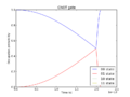
[[File:Rotation coeffs.png|border|600px]] |
|||
Above is a graph of the 4 values as a function of <math>\Delta_1</math>. If we wish to consider the regime in which <math>\Delta_1>\Delta_2</math> as above, we should consider the part of the graph to the right of the black dotted line. |
|||
A few qualitative statements can be made about the logical gates based off of this graph. First, it is clear that the <math>X_2</math> gate will always be faster than the <math>X_1</math> gate. A feature of concern is the behavior of <math>C_2</math>, namely that it tends towards zero, as this increases the time for the <math>\text{CNOT}_2</math> gate. |
|||
===Numerical Simulations=== |
|||
[[Image:x1 gate.gif|thumb|200px|Animation of the density matrix during the application of the X1 gate]] |
|||
[[Image:x2 gate.gif|thumb|200px|Animation of the density matrix during the application of the X2 gate]] |
|||
Using the QuTiP package, we can simulate the Master Equation for the system in question. First, we can verify the gates that we proposed under ideal conditions. Below are pictures of the density matrix as it undergoes pulses that we have predicted to correspond to X1 and X2 gates. Note that the behavior of the density matrix matches what we would expect. |
|||
<gallery> |
|||
File:X1 00.png|Beginning of X1 Gate |
|||
File:X1 99.png|End of X1 Gate |
|||
File:X2 00.png|Beginning of X2 Gate |
|||
File:X2 99.png|End of X2 Gate |
|||
</gallery> |
|||
Animations of these transformations can be found on the right. |
|||
Issues with CNOT gate: |
|||
<gallery> |
|||
File:State population oscillations 00 state.png|00 state |
|||
File:State population oscillations 10 state.png|10 state |
|||
File:State population oscillations super.png|Superpostition between 00 and 01 state |
|||
</gallery> |
|||
Latest revision as of 15:56, 2 December 2014
This project started in the Fall of 2014, focusing on the operation of two or more charge qubits which are capacitively coupled. Current PDF Summary can be found File:Capacitively Coupled Qubits.pdf
General Formulation

For a single charge qubit, the Hamiltonian is

We will refer to and as the detuning and tunnel coupling of qubit , respectively.


We can further write down the full Hamiltonian explicitly:

where is the capacitive coupling between the qubits.

Sweet Spots
A major issue with charge qubits is that they are very susceptible to charge noise, which occurs when charge fluctuations outside the system induce undesired shifts in the parameters of the Hamiltonian. The goal of a sweet spot is to find a point in the parameter space where the energy levels are as invariant to the shifts as possible.
First Order Detuning Noise
The most dominant noise source is due to the shifts in the detuning. It is believed that the only point at which the first order dependence on the detunings disappears is at . This has been confirmed analytically in the limit of small , and no exceptions have been observed numerically.

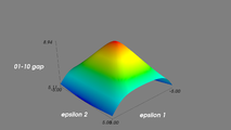
Gap between 01 and 10 states
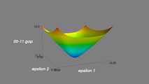
Gap between 00 and 11 states
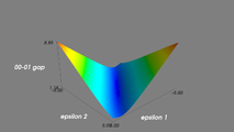
Gap between 00 and 01 states
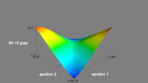
Gap between 00 and 10 states


Second Order Detuning Noise
For , we have the following energy levels:


which to second order in are:


The second order terms cannot be tuned such that all gaps are invariant to second order noise. However, can be tuned such that some of the transitions become invariant to some of the second order detuning shifts. To make the transition between and flat with respect to second order fluctuations in , we can set


Unfortunately, none of the other transitions can be made to be invariant to second order fluctuations in . Also, If we wish to make this transition invariant to all second order detuning fluctuations, we must set , making .


Tunnel Coupling and Capacitive Coupling Noise


Assuming that we sit at the sweet spot , the energies are relatively simple, so we can easily see the effect of noise on the other parameters.
| State | Energy | Effect of | Effect of |
|---|---|---|---|


Note that if we want any of the transitions to be invariant to first-order fluctuations in tunnel coupling, we would need to set either or to zero or set . The first change would make the energy levels degenerate, which must be avoided. If we set the tunnel couplings to be equal, it would be impossible to make any of the transitions invariant to second order effects in the detuning.


There is nothing we can do short of making the energy levels degenerate to make the transitions invariant with respect to first-order fluctuations in capacitive coupling. We could, however, make the coupling itself as stable as possible through manipulating the geometry of the system.
Rotations
Shifting to the Rotating Frame
After bringing the system adiabatically to the sweet spot , we can apply an AC pulse to some of our parameters to induce a rotation within the system.
| AC Pulse | Resulting Matrix (Lab Basis) | Resulting Matrix (Energy Basis) |
|---|---|---|


where , , and , , , and are all complicated functions of the parameters which are discussed below.


Based off of the rotation matrices in the energy basis, it's clear that the situation in which fundamentally differs from the case in which . Moreover, it can be seen that the case in which yields diverging results (as some of the matrix elements feature a step function at this point). So in practice, it would be good to avoid this point. Writing the rotations explicitly for the two regimes:


| AC Pulse | Energy Basis () | Energy Basis () |
|---|---|---|
| Failed to parse (SVG (MathML can be enabled via browser plugin): Invalid response ("Math extension cannot connect to Restbase.") from server "https://en.wikipedia.org/api/rest_v1/":): {\displaystyle \epsilon_2} | Failed to parse (SVG (MathML can be enabled via browser plugin): Invalid response ("Math extension cannot connect to Restbase.") from server "https://en.wikipedia.org/api/rest_v1/":): {\displaystyle \frac{1}{2}\left( \begin{matrix} 0 & -C_1 & -C_2 & 0 \\ -C_1 & 0 & 0 & C_2 \\ -C_2 & 0 & 0 & -C_1 \\ 0 & C_2 & -C_1 & 0 \end{matrix}\right)\cos{(\omega_{AC}t)}} | |
| Failed to parse (SVG (MathML can be enabled via browser plugin): Invalid response ("Math extension cannot connect to Restbase.") from server "https://en.wikipedia.org/api/rest_v1/":): {\displaystyle \frac{1}{2}\left( \begin{matrix} -B\frac{\Delta_1+\Delta_2}{\lambda_1} & 0 & 0 & -B\frac{g}{\lambda_1} \\ 0 & -B\frac{\Delta_1-\Delta_2}{\lambda_2} & -B\frac{g}{\lambda_2} & 0 \\ 0& -B\frac{g}{\lambda_2} & B\frac{\Delta_1-\Delta_2}{\lambda_2} & 0\\ -B\frac{g}{\lambda_1}& 0 & 0 &B\frac{\Delta_1+\Delta_2}{\lambda_1} \end{matrix}\right)\cos{(\omega_{AC}t)}} | Failed to parse (SVG (MathML can be enabled via browser plugin): Invalid response ("Math extension cannot connect to Restbase.") from server "https://en.wikipedia.org/api/rest_v1/":): {\displaystyle \frac{1}{2}\left( \begin{matrix} -B\frac{\Delta_1+\Delta_2}{\lambda_1} & 0 & 0 & -B\frac{g}{\lambda_1} \\ 0 & -B\frac{\Delta_1-\Delta_2}{\lambda_2} & B\frac{g}{\lambda_2} & 0 \\ 0& B\frac{g}{\lambda_2} & B\frac{\Delta_1-\Delta_2}{\lambda_2} & 0\\ -B\frac{g}{\lambda_1}& 0 & 0 &B\frac{\Delta_1+\Delta_2}{\lambda_1} \end{matrix}\right)\cos{(\omega_{AC}t)}} | |
| Failed to parse (SVG (MathML can be enabled via browser plugin): Invalid response ("Math extension cannot connect to Restbase.") from server "https://en.wikipedia.org/api/rest_v1/":): {\displaystyle \Delta_2} | Failed to parse (SVG (MathML can be enabled via browser plugin): Invalid response ("Math extension cannot connect to Restbase.") from server "https://en.wikipedia.org/api/rest_v1/":): {\displaystyle \frac{1}{2}\left( \begin{matrix} -B\frac{\Delta_1+\Delta_2}{\lambda_1} & 0 & 0 & -B\frac{g}{\lambda_1} \\ 0 & B\frac{\Delta_1-\Delta_2}{\lambda_2} & B\frac{g}{\lambda_2} & 0 \\ 0 & B\frac{g}{\lambda_2} & -B\frac{\Delta_1-\Delta_2}{\lambda_2} & 0 \\ -B\frac{g}{\lambda_1}& 0 & 0 &B\frac{\Delta_1+\Delta_2}{\lambda_1} \end{matrix}\right)\cos{(\omega_{AC}t)}} | Failed to parse (SVG (MathML can be enabled via browser plugin): Invalid response ("Math extension cannot connect to Restbase.") from server "https://en.wikipedia.org/api/rest_v1/":): {\displaystyle \frac{1}{2}\left( \begin{matrix} -B\frac{\Delta_1+\Delta_2}{\lambda_1} & 0 & 0 & -B\frac{g}{\lambda_1} \\ 0 & B\frac{\Delta_1-\Delta_2}{\lambda_2} & -B\frac{g}{\lambda_2} & 0 \\ 0 & -B\frac{g}{\lambda_2} & -B\frac{\Delta_1-\Delta_2}{\lambda_2} & 0 \\ -B\frac{g}{\lambda_1}& 0 & 0 &B\frac{\Delta_1+\Delta_2}{\lambda_1} \end{matrix}\right)\cos{(\omega_{AC}t)}} |


We can further analyze these matrices by considering the effective rotations in the rotating frame for different applied frequencies, using the rotating wave approximation:
| AC Pulse | Rotating Frame (Failed to parse (SVG (MathML can be enabled via browser plugin): Invalid response ("Math extension cannot connect to Restbase.") from server "https://en.wikipedia.org/api/rest_v1/":): {\displaystyle \Delta_1>\Delta_2} ) | Rotating Frame (Failed to parse (SVG (MathML can be enabled via browser plugin): Invalid response ("Math extension cannot connect to Restbase.") from server "https://en.wikipedia.org/api/rest_v1/":): {\displaystyle \Delta_1<\Delta_2} ) | |
|---|---|---|---|
| Failed to parse (SVG (MathML can be enabled via browser plugin): Invalid response ("Math extension cannot connect to Restbase.") from server "https://en.wikipedia.org/api/rest_v1/":): {\displaystyle \epsilon_1} | Failed to parse (SVG (MathML can be enabled via browser plugin): Invalid response ("Math extension cannot connect to Restbase.") from server "https://en.wikipedia.org/api/rest_v1/":): {\displaystyle \omega_{AC} = (\lambda_1-\lambda_2)/\hbar} | Failed to parse (SVG (MathML can be enabled via browser plugin): Invalid response ("Math extension cannot connect to Restbase.") from server "https://en.wikipedia.org/api/rest_v1/":): {\displaystyle \frac{1}{4}\left( \begin{matrix} 0 & A_1 & 0 & 0 \\ A_1 & 0 & 0 & 0 \\ 0 & 0 & 0 & -A_1 \\ 0 & 0 & -A_1 & 0 \end{matrix}\right)} | Failed to parse (SVG (MathML can be enabled via browser plugin): Invalid response ("Math extension cannot connect to Restbase.") from server "https://en.wikipedia.org/api/rest_v1/":): {\displaystyle \frac{1}{4}\left( \begin{matrix} 0 & -A_1 & 0 & 0 \\ -A_1 & 0 & 0 & 0 \\ 0 & 0 & 0 & -A_1 \\ 0 & 0 & -A_1 & 0 \end{matrix}\right)} |
| Failed to parse (SVG (MathML can be enabled via browser plugin): Invalid response ("Math extension cannot connect to Restbase.") from server "https://en.wikipedia.org/api/rest_v1/":): {\displaystyle \omega_{AC} = (\lambda_1+\lambda_2)/\hbar} | Failed to parse (SVG (MathML can be enabled via browser plugin): Invalid response ("Math extension cannot connect to Restbase.") from server "https://en.wikipedia.org/api/rest_v1/":): {\displaystyle \frac{1}{4}\left( \begin{matrix} 0 & 0 & -A_2 & 0 \\ 0 & 0 & 0 & -A_2 \\ -A_2 & 0 & 0 & 0 \\ 0 & -A_2 & 0 & 0 \end{matrix}\right)} | Failed to parse (SVG (MathML can be enabled via browser plugin): Invalid response ("Math extension cannot connect to Restbase.") from server "https://en.wikipedia.org/api/rest_v1/":): {\displaystyle \frac{1}{4}\left( \begin{matrix} 0 & 0 & -A_2 & 0 \\ 0 & 0 & 0 & A_2 \\ -A_2 & 0 & 0 & 0 \\ 0 & A_2 & 0 & 0 \end{matrix}\right)} | |
| Failed to parse (SVG (MathML can be enabled via browser plugin): Invalid response ("Math extension cannot connect to Restbase.") from server "https://en.wikipedia.org/api/rest_v1/":): {\displaystyle \epsilon_2} | Failed to parse (SVG (MathML can be enabled via browser plugin): Invalid response ("Math extension cannot connect to Restbase.") from server "https://en.wikipedia.org/api/rest_v1/":): {\displaystyle \omega_{AC} = (\lambda_1-\lambda_2)/\hbar} | Failed to parse (SVG (MathML can be enabled via browser plugin): Invalid response ("Math extension cannot connect to Restbase.") from server "https://en.wikipedia.org/api/rest_v1/":): {\displaystyle \frac{1}{4}\left( \begin{matrix} 0 & -C_1 & 0 & 0 \\ -C_1 & 0 & 0 & 0 \\ 0 & 0 & 0 & -C_1 \\ 0 & 0 & -C_1 & 0 \end{matrix}\right)} | Failed to parse (SVG (MathML can be enabled via browser plugin): Invalid response ("Math extension cannot connect to Restbase.") from server "https://en.wikipedia.org/api/rest_v1/":): {\displaystyle \frac{1}{4}\left( \begin{matrix} 0 & C_1 & 0 & 0 \\ C_1 & 0 & 0 & 0 \\ 0 & 0 & 0 & -C_1 \\ 0 & 0 & -C_1 & 0 \end{matrix}\right)} |
| Failed to parse (SVG (MathML can be enabled via browser plugin): Invalid response ("Math extension cannot connect to Restbase.") from server "https://en.wikipedia.org/api/rest_v1/":): {\displaystyle \omega_{AC} = (\lambda_1+\lambda_2)/\hbar} | Failed to parse (SVG (MathML can be enabled via browser plugin): Invalid response ("Math extension cannot connect to Restbase.") from server "https://en.wikipedia.org/api/rest_v1/":): {\displaystyle \frac{1}{4}\left( \begin{matrix} 0 & 0 & -C_2 & 0 \\ 0 & 0 & 0 & C_2 \\ -C_2 & 0 & 0 & 0 \\ 0 & C_2 & 0 & 0 \end{matrix}\right)} | Failed to parse (SVG (MathML can be enabled via browser plugin): Invalid response ("Math extension cannot connect to Restbase.") from server "https://en.wikipedia.org/api/rest_v1/":): {\displaystyle \frac{1}{4}\left( \begin{matrix} 0 & 0 & -C_2 & 0 \\ 0 & 0 & 0 & -C_2 \\ -C_2 & 0 & 0 & 0 \\ 0 & -C_2 & 0 & 0 \end{matrix}\right)} | |
| Failed to parse (SVG (MathML can be enabled via browser plugin): Invalid response ("Math extension cannot connect to Restbase.") from server "https://en.wikipedia.org/api/rest_v1/":): {\displaystyle \Delta_1} | Failed to parse (SVG (MathML can be enabled via browser plugin): Invalid response ("Math extension cannot connect to Restbase.") from server "https://en.wikipedia.org/api/rest_v1/":): {\displaystyle \omega_{AC} = 2(\lambda_1)/\hbar} | Failed to parse (SVG (MathML can be enabled via browser plugin): Invalid response ("Math extension cannot connect to Restbase.") from server "https://en.wikipedia.org/api/rest_v1/":): {\displaystyle \frac{1}{4}\left( \begin{matrix} 0 & 0 & 0 & -B\frac{g}{\lambda_1} \\ 0 & 0 & 0 & 0 \\ 0& 0 & 0 & 0\\ -B\frac{g}{\lambda_1}& 0 & 0 &0 \end{matrix}\right)} | Failed to parse (SVG (MathML can be enabled via browser plugin): Invalid response ("Math extension cannot connect to Restbase.") from server "https://en.wikipedia.org/api/rest_v1/":): {\displaystyle \frac{1}{4}\left( \begin{matrix} 0 & 0 & 0 & -B\frac{g}{\lambda_1} \\ 0 & 0 & 0 & 0 \\ 0& 0 & 0 & 0\\ -B\frac{g}{\lambda_1}& 0 & 0 &0 \end{matrix}\right)} |
| Failed to parse (SVG (MathML can be enabled via browser plugin): Invalid response ("Math extension cannot connect to Restbase.") from server "https://en.wikipedia.org/api/rest_v1/":): {\displaystyle \omega_{AC} = 2(\lambda_2)/\hbar} | Failed to parse (SVG (MathML can be enabled via browser plugin): Invalid response ("Math extension cannot connect to Restbase.") from server "https://en.wikipedia.org/api/rest_v1/":): {\displaystyle \frac{1}{4}\left( \begin{matrix} 0 & 0 & 0 & 0 \\ 0 & 0 & -B\frac{g}{\lambda_2} & 0 \\ 0& -B\frac{g}{\lambda_2} & 0 & 0\\ 0& 0 & 0 &0 \end{matrix}\right)} | Failed to parse (SVG (MathML can be enabled via browser plugin): Invalid response ("Math extension cannot connect to Restbase.") from server "https://en.wikipedia.org/api/rest_v1/":): {\displaystyle \frac{1}{4}\left( \begin{matrix} 0 & 0 & 0 &0 \\ 0 & 0 & B\frac{g}{\lambda_2} & 0 \\ 0& B\frac{g}{\lambda_2} & 0 & 0\\ 0& 0 & 0 &0 \end{matrix}\right)} | |
| Failed to parse (SVG (MathML can be enabled via browser plugin): Invalid response ("Math extension cannot connect to Restbase.") from server "https://en.wikipedia.org/api/rest_v1/":): {\displaystyle \Delta_2} | Failed to parse (SVG (MathML can be enabled via browser plugin): Invalid response ("Math extension cannot connect to Restbase.") from server "https://en.wikipedia.org/api/rest_v1/":): {\displaystyle \omega_{AC} = 2(\lambda_1)/\hbar} | Failed to parse (SVG (MathML can be enabled via browser plugin): Invalid response ("Math extension cannot connect to Restbase.") from server "https://en.wikipedia.org/api/rest_v1/":): {\displaystyle \frac{1}{4}\left( \begin{matrix} 0 & 0 & 0 & -B\frac{g}{\lambda_1} \\ 0 & 0 & 0 & 0 \\ 0 & 0 & 0 & 0 \\ -B\frac{g}{\lambda_1}& 0 & 0 &0 \end{matrix}\right)} | Failed to parse (SVG (MathML can be enabled via browser plugin): Invalid response ("Math extension cannot connect to Restbase.") from server "https://en.wikipedia.org/api/rest_v1/":): {\displaystyle \frac{1}{4}\left( \begin{matrix} 0 & 0 & 0 & -B\frac{g}{\lambda_1} \\ 0 & 0 & 0 & 0 \\ 0 & 0 & 0 & 0 \\ -B\frac{g}{\lambda_1}& 0 & 0 &0 \end{matrix}\right)} |
| Failed to parse (SVG (MathML can be enabled via browser plugin): Invalid response ("Math extension cannot connect to Restbase.") from server "https://en.wikipedia.org/api/rest_v1/":): {\displaystyle \omega_{AC} = 2(\lambda_2)/\hbar} | Failed to parse (SVG (MathML can be enabled via browser plugin): Invalid response ("Math extension cannot connect to Restbase.") from server "https://en.wikipedia.org/api/rest_v1/":): {\displaystyle \frac{1}{4}\left( \begin{matrix} 0 & 0 & 0 & 0 \\ 0 & 0 & B\frac{g}{\lambda_2} & 0 \\ 0 & B\frac{g}{\lambda_2} & 0 & 0 \\ 0& 0 & 0 &0 \end{matrix}\right)} | Failed to parse (SVG (MathML can be enabled via browser plugin): Invalid response ("Math extension cannot connect to Restbase.") from server "https://en.wikipedia.org/api/rest_v1/":): {\displaystyle \frac{1}{4}\left( \begin{matrix} 0 & 0 & 0 & 0 \\ 0 & 0 & -B\frac{g}{\lambda_2} & 0 \\ 0 & -B\frac{g}{\lambda_2} & 0 & 0 \\ 0& 0 & 0 &0 \end{matrix}\right)} | |
Constructing Logical Gates
We will assume in this section that we are in the regime Failed to parse (SVG (MathML can be enabled via browser plugin): Invalid response ("Math extension cannot connect to Restbase.") from server "https://en.wikipedia.org/api/rest_v1/":): {\displaystyle \Delta_1>\Delta_2} . The same gates can be determined in the other regime as well.
- Failed to parse (SVG (MathML can be enabled via browser plugin): Invalid response ("Math extension cannot connect to Restbase.") from server "https://en.wikipedia.org/api/rest_v1/":): {\displaystyle Z_1}
gate (Failed to parse (SVG (MathML can be enabled via browser plugin): Invalid response ("Math extension cannot connect to Restbase.") from server "https://en.wikipedia.org/api/rest_v1/":): {\displaystyle Z}
on qubit 1)
- Wait for a time Failed to parse (SVG (MathML can be enabled via browser plugin): Invalid response ("Math extension cannot connect to Restbase.") from server "https://en.wikipedia.org/api/rest_v1/":): {\displaystyle \tau = \frac{h}{2(\lambda_1+\lambda_2)}} (always on)
- Failed to parse (SVG (MathML can be enabled via browser plugin): Invalid response ("Math extension cannot connect to Restbase.") from server "https://en.wikipedia.org/api/rest_v1/":): {\displaystyle Z_2}
gate (Failed to parse (SVG (MathML can be enabled via browser plugin): Invalid response ("Math extension cannot connect to Restbase.") from server "https://en.wikipedia.org/api/rest_v1/":): {\displaystyle Z}
on qubit 2)
- Wait for a time Failed to parse (SVG (MathML can be enabled via browser plugin): Invalid response ("Math extension cannot connect to Restbase.") from server "https://en.wikipedia.org/api/rest_v1/":): {\displaystyle \tau = \frac{h}{2(\lambda_1-\lambda_2)}} (always on)
- Failed to parse (SVG (MathML can be enabled via browser plugin): Invalid response ("Math extension cannot connect to Restbase.") from server "https://en.wikipedia.org/api/rest_v1/":): {\displaystyle X_1}
gate (Failed to parse (SVG (MathML can be enabled via browser plugin): Invalid response ("Math extension cannot connect to Restbase.") from server "https://en.wikipedia.org/api/rest_v1/":): {\displaystyle X}
on qubit 1)
- Pulse Failed to parse (SVG (MathML can be enabled via browser plugin): Invalid response ("Math extension cannot connect to Restbase.") from server "https://en.wikipedia.org/api/rest_v1/":): {\displaystyle \epsilon_1} at a frequency of Failed to parse (SVG (MathML can be enabled via browser plugin): Invalid response ("Math extension cannot connect to Restbase.") from server "https://en.wikipedia.org/api/rest_v1/":): {\displaystyle \omega_{AC} = (\lambda_1+\lambda_2)/\hbar} for a time Failed to parse (SVG (MathML can be enabled via browser plugin): Invalid response ("Math extension cannot connect to Restbase.") from server "https://en.wikipedia.org/api/rest_v1/":): {\displaystyle \tau = \frac{2h}{A_2}}
- Failed to parse (SVG (MathML can be enabled via browser plugin): Invalid response ("Math extension cannot connect to Restbase.") from server "https://en.wikipedia.org/api/rest_v1/":): {\displaystyle X_2}
gate (Failed to parse (SVG (MathML can be enabled via browser plugin): Invalid response ("Math extension cannot connect to Restbase.") from server "https://en.wikipedia.org/api/rest_v1/":): {\displaystyle X}
on qubit 2)
- Pulse Failed to parse (SVG (MathML can be enabled via browser plugin): Invalid response ("Math extension cannot connect to Restbase.") from server "https://en.wikipedia.org/api/rest_v1/":): {\displaystyle \epsilon_2} at a frequency of Failed to parse (SVG (MathML can be enabled via browser plugin): Invalid response ("Math extension cannot connect to Restbase.") from server "https://en.wikipedia.org/api/rest_v1/":): {\displaystyle \omega_{AC} = (\lambda_1-\lambda_2)/\hbar} for a time Failed to parse (SVG (MathML can be enabled via browser plugin): Invalid response ("Math extension cannot connect to Restbase.") from server "https://en.wikipedia.org/api/rest_v1/":): {\displaystyle \tau = \frac{2h}{C_1}}
- Failed to parse (SVG (MathML can be enabled via browser plugin): Invalid response ("Math extension cannot connect to Restbase.") from server "https://en.wikipedia.org/api/rest_v1/":): {\displaystyle \text{CNOT}_1}
gate (Failed to parse (SVG (MathML can be enabled via browser plugin): Invalid response ("Math extension cannot connect to Restbase.") from server "https://en.wikipedia.org/api/rest_v1/":): {\displaystyle \text{CNOT}}
with qubit 1 as control)
- Pulse Failed to parse (SVG (MathML can be enabled via browser plugin): Invalid response ("Math extension cannot connect to Restbase.") from server "https://en.wikipedia.org/api/rest_v1/":): {\displaystyle \epsilon_1} at a frequency of Failed to parse (SVG (MathML can be enabled via browser plugin): Invalid response ("Math extension cannot connect to Restbase.") from server "https://en.wikipedia.org/api/rest_v1/":): {\displaystyle \omega_{AC} = (\lambda_1-\lambda_2)/\hbar} for a time Failed to parse (SVG (MathML can be enabled via browser plugin): Invalid response ("Math extension cannot connect to Restbase.") from server "https://en.wikipedia.org/api/rest_v1/":): {\displaystyle \tau = \frac{h}{A_1}}
- Pulse Failed to parse (SVG (MathML can be enabled via browser plugin): Invalid response ("Math extension cannot connect to Restbase.") from server "https://en.wikipedia.org/api/rest_v1/":): {\displaystyle \epsilon_2} at a frequency of Failed to parse (SVG (MathML can be enabled via browser plugin): Invalid response ("Math extension cannot connect to Restbase.") from server "https://en.wikipedia.org/api/rest_v1/":): {\displaystyle \omega_{AC} = (\lambda_1-\lambda_2)/\hbar} for a time Failed to parse (SVG (MathML can be enabled via browser plugin): Invalid response ("Math extension cannot connect to Restbase.") from server "https://en.wikipedia.org/api/rest_v1/":): {\displaystyle \tau = \frac{h}{C_1}}
- Failed to parse (SVG (MathML can be enabled via browser plugin): Invalid response ("Math extension cannot connect to Restbase.") from server "https://en.wikipedia.org/api/rest_v1/":): {\displaystyle \text{CNOT}_2}
gate (Failed to parse (SVG (MathML can be enabled via browser plugin): Invalid response ("Math extension cannot connect to Restbase.") from server "https://en.wikipedia.org/api/rest_v1/":): {\displaystyle \text{CNOT}}
with qubit 2 as control)
- Pulse Failed to parse (SVG (MathML can be enabled via browser plugin): Invalid response ("Math extension cannot connect to Restbase.") from server "https://en.wikipedia.org/api/rest_v1/":): {\displaystyle \epsilon_2} at a frequency of Failed to parse (SVG (MathML can be enabled via browser plugin): Invalid response ("Math extension cannot connect to Restbase.") from server "https://en.wikipedia.org/api/rest_v1/":): {\displaystyle \omega_{AC} = (\lambda_1+\lambda_2)/\hbar} for a time Failed to parse (SVG (MathML can be enabled via browser plugin): Invalid response ("Math extension cannot connect to Restbase.") from server "https://en.wikipedia.org/api/rest_v1/":): {\displaystyle \tau = \frac{h}{C_2}}
- Pulse at a frequency of for a time
-
- Pulse either or at a frequency of for a time


Notes on Logical Operating Points
Here we discuss the values of , , , and . Analytical expressions can and have been found for these quantities, but they yield little intuition about their nature.

Above is a graph of the 4 values as a function of . If we wish to consider the regime in which as above, we should consider the part of the graph to the right of the black dotted line.
A few qualitative statements can be made about the logical gates based off of this graph. First, it is clear that the gate will always be faster than the gate. A feature of concern is the behavior of , namely that it tends towards zero, as this increases the time for the gate.


Numerical Simulations


Using the QuTiP package, we can simulate the Master Equation for the system in question. First, we can verify the gates that we proposed under ideal conditions. Below are pictures of the density matrix as it undergoes pulses that we have predicted to correspond to X1 and X2 gates. Note that the behavior of the density matrix matches what we would expect.

Beginning of X1 Gate
End of X1 Gate
Beginning of X2 Gate
End of X2 Gate


Animations of these transformations can be found on the right.
Issues with CNOT gate:
00 state

10 state
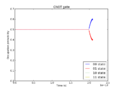
Superpostition between 00 and 01 state


